Eigenvalue falls in thin broken quantum strips
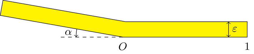
We consider the spectrum of the Dirichlet Laplacian in thin broken strips with angle \(\alpha\) and width \(\varepsilon>0\) as above.
For \(\alpha=0\), the eigenvalues and corresponding eigenfunctions are simply
\begin{equation}
\cfrac{m^2\pi^2}{\varepsilon^2}+\cfrac{n^2\pi^2}{4},\qquad\quad \sin(m\pi y/\varepsilon)\sin(n\pi(x+1)/2).
\end{equation}
For \(\alpha\ne0\), we give an asymptotic expansion of the first eigenvalues and corresponding eigenfunctions as \(\varepsilon\) tends to zero.
In particular, we study the dependence of the eigenpairs with respect to \(\alpha\).
For a small fixed \(\varepsilon>0\), at certain particular angles \(\alpha_k\), \(k = 0, 1,\dots\), that we can characterize, an eigenvalue dives,
i.e. moves down rapidly, below the normalized threshold \(\pi^2/\varepsilon^2\) as \(\alpha>0\) increases.
This phenomenon can be observed on the graphs below where we display the eigenvalues with respect to \(\alpha\)
(the right picture is a zoom of the left around \(\alpha=1.4\) and the red dotted line marks the value \(\pi^2/\varepsilon^2\)).

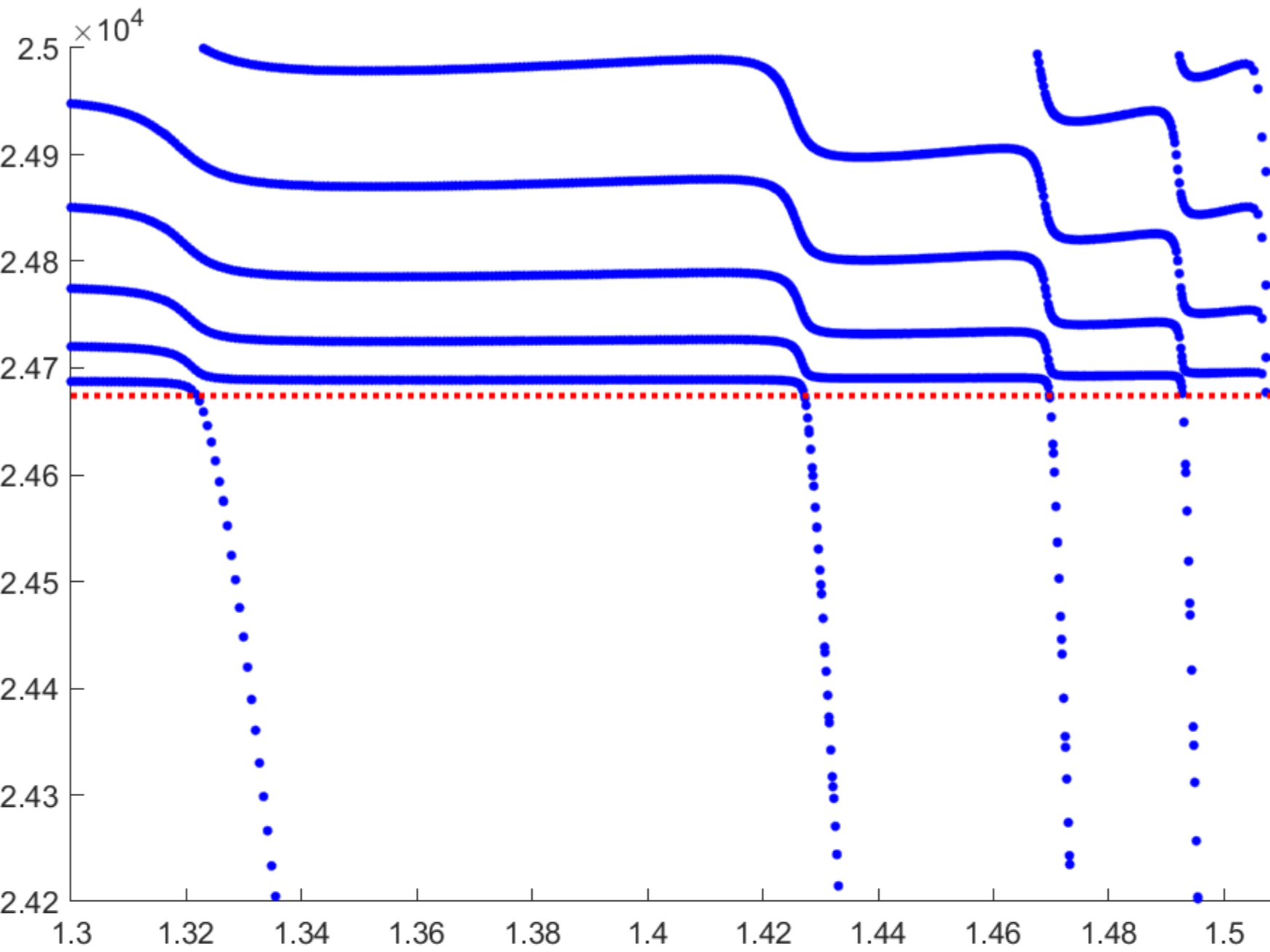
We can describe the way the eigenvalue dives below \(\pi^2/\varepsilon^2\) and prove that the phenomenon is milder at \(\alpha_0=0\) than at \(\alpha_k\) for \(k \ge 1\). In the process, the shape of the corresponding eigenfunctions exhibit a drastic change as illustrated on the movies 1 and 3 below. More details in [PDF].
We can describe the way the eigenvalue dives below \(\pi^2/\varepsilon^2\) and prove that the phenomenon is milder at \(\alpha_0=0\) than at \(\alpha_k\) for \(k \ge 1\). In the process, the shape of the corresponding eigenfunctions exhibit a drastic change as illustrated on the movies 1 and 3 below. More details in [PDF].
\( \hspace{1.6cm} \mbox{Eigenfunction 1} \hspace{3.2cm} \mbox{Eigenfunction 2} \hspace{3.2cm} \mbox{Eigenfunction 3} \)
Breath of the spectrum of the Dirichlet Laplacian in thin periodic waveguides
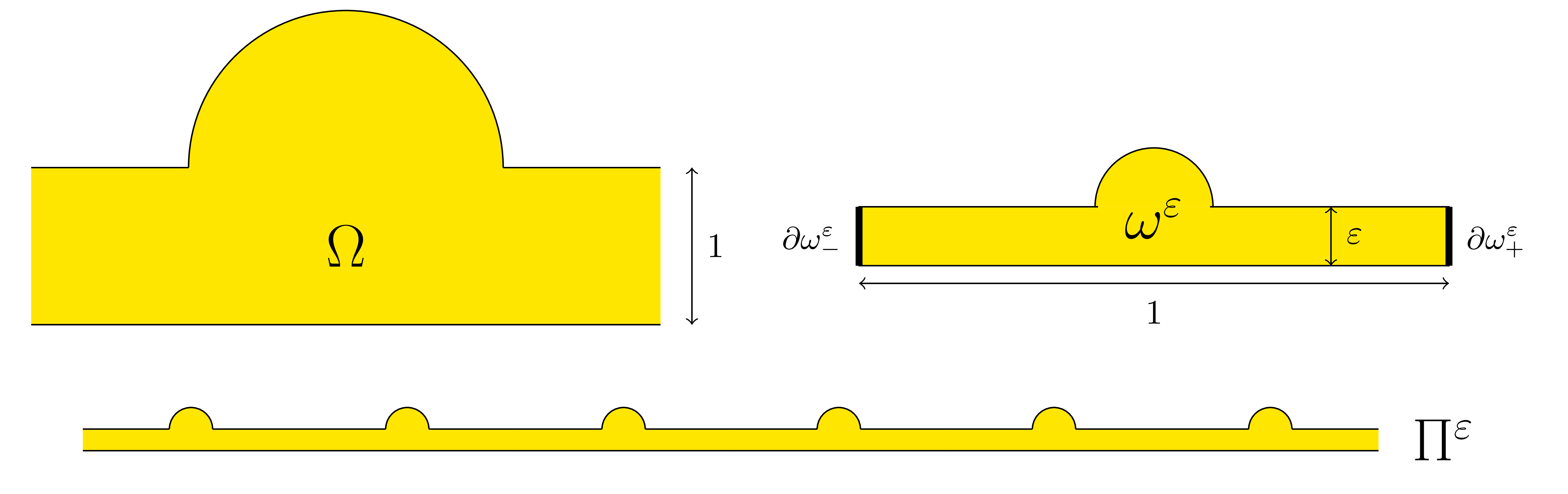
Let \(\Omega\) be a waveguide which coincides with the strip \(\mathbb{R}\times(-1/2;1/2)\) outside of a bounded region.
From it, define for \(\varepsilon>0\) small the thin periodicity cell \(\omega^\varepsilon:=\{(x,y)\,|\,(x/\varepsilon,y/\varepsilon)\in\Omega, |x|<1/2\}\).
Finally repeat periodically this pattern along the \(x\)-direction to create the thin periodic waveguide \(\Pi^\varepsilon\).
In \(\Pi^\varepsilon\), we consider the spectrum of the Dirichlet Laplacian \(A^\varepsilon\), that we denote by \(\sigma(A^\varepsilon)\). In other words, we study the spectral problem
\begin{equation}
\begin{array}{|rcll}
-\Delta u &=&\lambda u &\mbox{ in }\Pi^\varepsilon\\[3pt]
u &=& 0 &\mbox{ on }\Pi^\varepsilon.
\end{array}
\end{equation}
Due to the periodicity, it is known that \(\sigma(A^\varepsilon)\) has a band gap structure:
\begin{equation}
\sigma(A^\varepsilon)=\bigcup_{p\in\mathbb{N}^\ast}\Upsilon^\varepsilon_p
\end{equation}
where the \(\Upsilon^\varepsilon_p\) are compact intervals of \(\mathbb{R}\).
Classicaly, we have \(\Upsilon^\varepsilon_p=\bigcup_{\eta\in[0;2\pi)}\nu_p(\eta)\) where \(\nu_p(\eta)\) is the \(p-th\) eigenvalue of a spectral problem set in \(\omega^\varepsilon\) and involving quasi-periodic conditions at \(\partial\omega_\pm^\varepsilon\).
Below we represent we dispersion curves \(\eta\mapsto\nu_p(\eta)\) for some given \(\Omega\) and \(\varepsilon=0.1\).
The spectrum \(\sigma(A^\varepsilon)\) should be read on the vertical axis.
Due to the Dirichlet boundary conditions, all the bands \(\Upsilon^\varepsilon_p\) go to \(+\infty\) as \(\varepsilon^{-2}\) when \(\varepsilon\to0\).
Concerning the width of the \(\Upsilon^\varepsilon_p\), we obtain two types of behaviours.
The important message is that the features of the near field operator \(A^{\Omega}\), the Dirichlet Laplacian in \(\Omega\), play a key role in the results.
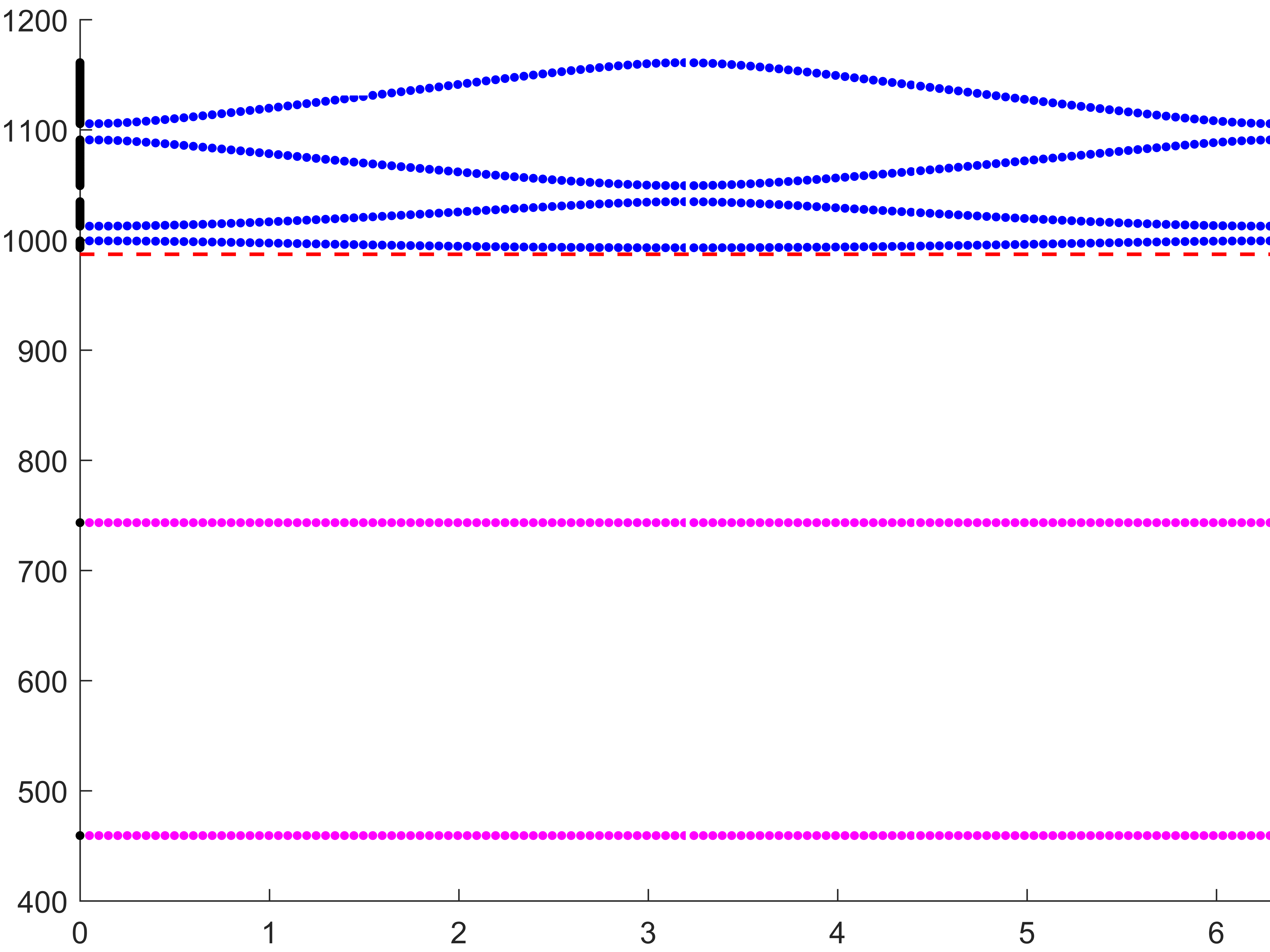
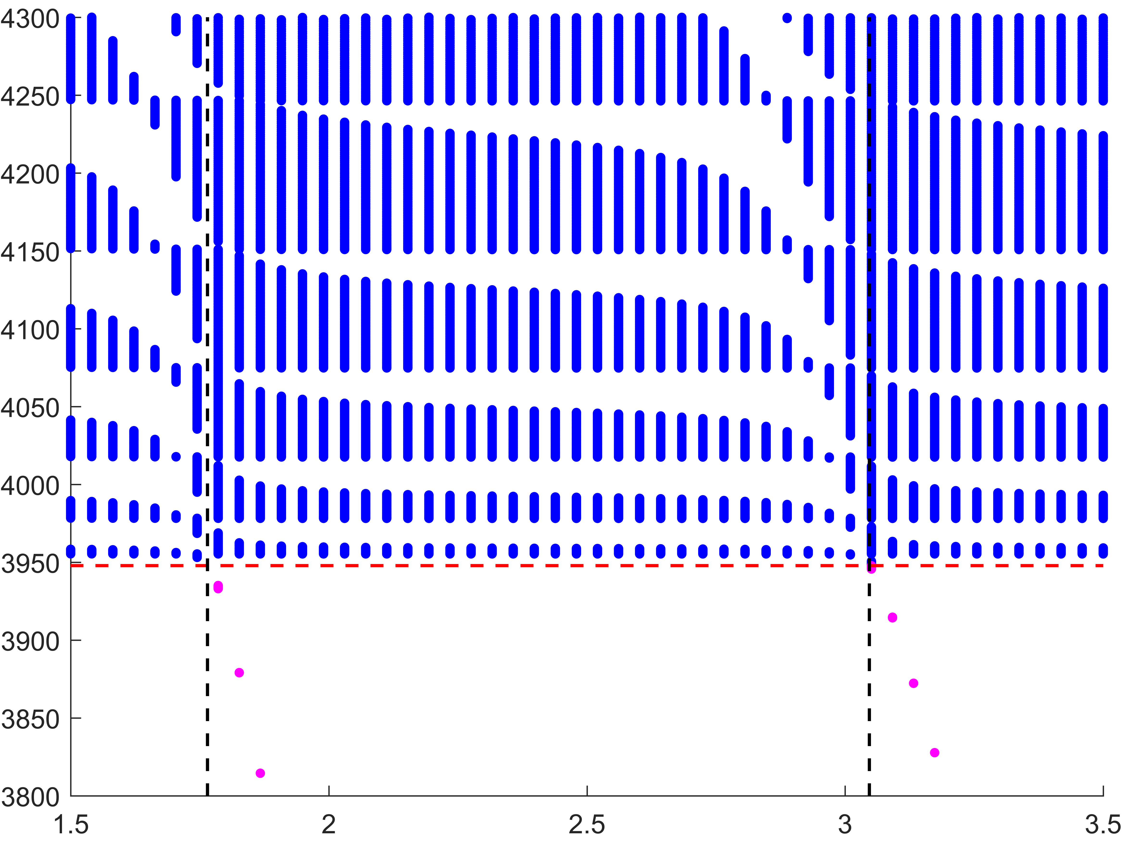
Below we represent \(\sigma(A^\varepsilon)\) with respect to \(H\) for \(\varepsilon=0.05\). The horizontal red line indicates the value \(\pi^2/\varepsilon^2\) while the vertical black lines mark the particular \(H=H_\star\) such that \(\mbox{dim}\,X_{\dagger}=1\). We see that when \(H\) approaches \(H_\star\), \(\sigma(A^\varepsilon)\) suddenly expands. Additionally, this breathing phenomenon gives birth to an extremely short spectral band (in magenta) which goes down below the critical value \(\pi^2/\varepsilon^2\).
Note that the properties of the space \(X_{\dagger}\) appear naturally in the asymptotic procedure when matching inner field and far field behaviours. Roughly speaking, when \(X_{\dagger}=\{0\}\), one should impose Dirichlet conditions at the junctions points of the 1D limit waveguide obtained by taking the limit \(\varepsilon\to0\). For this reason, waves cannot propagate in \(\Pi^\varepsilon\). On the other hand, when \(\mbox{dim}\,X_{\dagger}=1\), one must impose generalized Kirchhoff transmission conditions which allow for waves propagation. More details in [PDF].
- The bands below \(\pi^2/\varepsilon^2\) are extremely tight, of length \(O(e^{-\delta/\varepsilon})\), \(\delta>0\). Their number coincides with the number of eigenvalues of \(A^{\Omega}\) below its essential spectrum \(\pi^2\).
- The width of the next \(\Upsilon^\varepsilon_p\) depends on the geometry of \(\Omega\) and more precisely on the dimension of the space \(X_{\dagger}\) of bounded functions satisfying the threshold problem
\begin{equation}
\begin{array}{|rcll}
-\Delta u &=&\pi^2 u &\mbox{ in }\Omega\\[3pt]
u &=& 0 &\mbox{ on }\Omega
\end{array}
\end{equation}
and which do not decay at infinity.
When \(\Omega\) is such that \(X_{\dagger}=\{0\}\), which is the generic situation, the length of the next \(\Upsilon^\varepsilon_p\) is in \(O(\varepsilon)\) and there are some gaps in \(O(1)\). In that case, for most of the spectral parameters, waves can not propagate in the periodic waveguide.
When \(\Omega\) is such that \(\mbox{dim}\,X_{\dagger}=1\), the length of the next spectral bands is in \(O(1)\) and so, they are much more possibilities for waves to propagate in \(\Pi^\varepsilon\).
Below we represent \(\sigma(A^\varepsilon)\) with respect to \(H\) for \(\varepsilon=0.05\). The horizontal red line indicates the value \(\pi^2/\varepsilon^2\) while the vertical black lines mark the particular \(H=H_\star\) such that \(\mbox{dim}\,X_{\dagger}=1\). We see that when \(H\) approaches \(H_\star\), \(\sigma(A^\varepsilon)\) suddenly expands. Additionally, this breathing phenomenon gives birth to an extremely short spectral band (in magenta) which goes down below the critical value \(\pi^2/\varepsilon^2\).
Note that the properties of the space \(X_{\dagger}\) appear naturally in the asymptotic procedure when matching inner field and far field behaviours. Roughly speaking, when \(X_{\dagger}=\{0\}\), one should impose Dirichlet conditions at the junctions points of the 1D limit waveguide obtained by taking the limit \(\varepsilon\to0\). For this reason, waves cannot propagate in \(\Pi^\varepsilon\). On the other hand, when \(\mbox{dim}\,X_{\dagger}=1\), one must impose generalized Kirchhoff transmission conditions which allow for waves propagation. More details in [PDF].
Acoustic cloaking with thin resonant ligaments
Above, we represent the total field (acoustic pressure) in a waveguide with an obstacle for a wave incoming from the left.
It is a movie with respect to the time (time harmonic regime).
The wavenumber is set so that one mode can propagate.
The reflection and transmission coefficients \(R,\,T\in\mathbb{C}\) depend on the shape of the obstacle.
Below we add two thin resonant ligaments of width \(\varepsilon\) to this geometry. Choosing carefully their positions and their lengths, we can get \(R^\varepsilon\approx0\) and \(T^\varepsilon\approx1\) as in the reference strip (third animation). An essential ingredient in the approach is to work around the resonance lengths of the ligaments to obtain effects of order one with geometrical perturbations of width \(\varepsilon\). More details in [PDF].
Below we add two thin resonant ligaments of width \(\varepsilon\) to this geometry. Choosing carefully their positions and their lengths, we can get \(R^\varepsilon\approx0\) and \(T^\varepsilon\approx1\) as in the reference strip (third animation). An essential ingredient in the approach is to work around the resonance lengths of the ligaments to obtain effects of order one with geometrical perturbations of width \(\varepsilon\). More details in [PDF].

Below we cloak two other obstacles. For the plumbing, the problem is especially difficult because the initial transmission is almost zero.

Phase shifter with thin resonant cloaking
Thin resonant ligaments can also be used to design phase shifters.
These are devices where the reflection is zero and the transmission can be any number on the unit circle of the complex plane.
According to the position and the length of the ligaments, the phase shift can be chosen as desired.
Here the geometry has been conceived to obtain a phase shift equal to \(\pi/4\).
Again, an essential ingredient in the approach is to work around the resonance lengths
of the ligaments to obtain effects of order one with geometrical perturbations of width \(\varepsilon\). More details in [PDF].
Enhancement of absorption
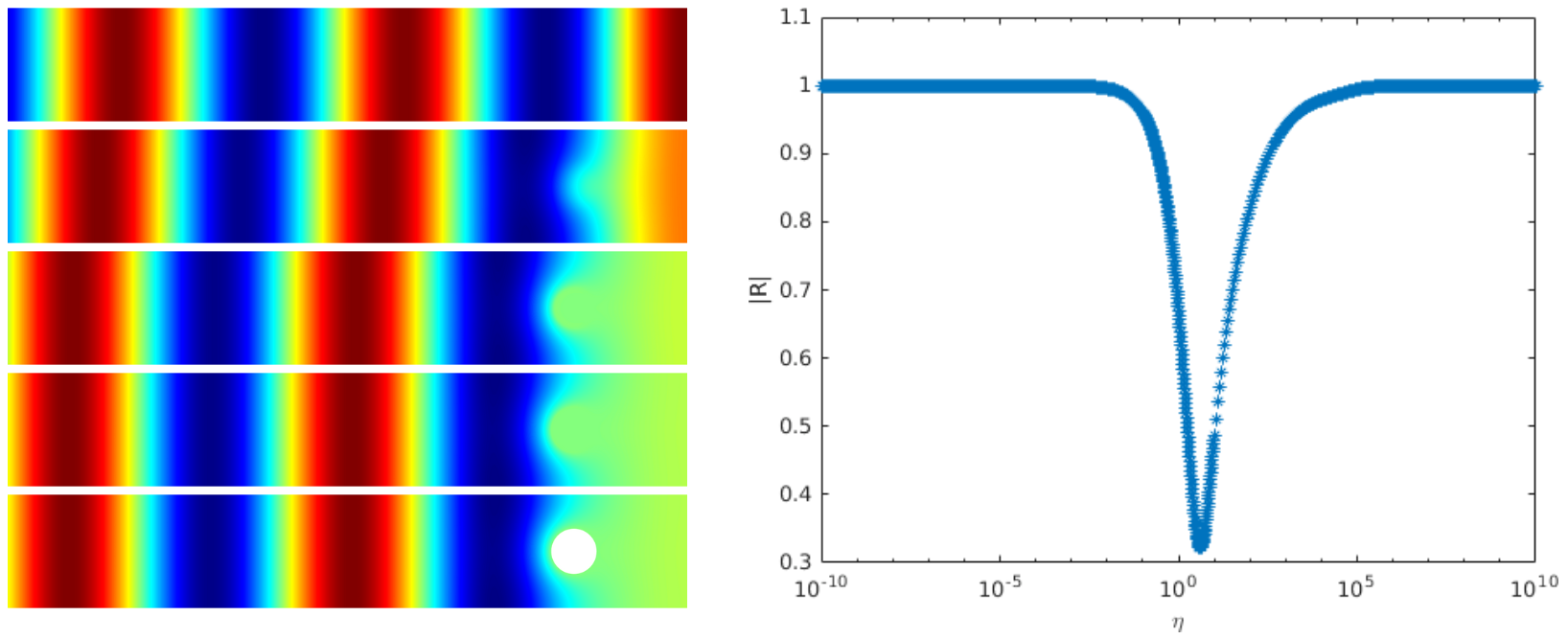
We consider the scattering of a plane wave coming from the left in an acoustic half-waveguide which contains a penetrable disk-shaped dissipative inclusion.
Dissipation is characterized by a parameter \(\eta\ge0\).
The frequency is set so that only one mode can propagate.
Hence the reflection matrix reduces to a complex number \(R^\eta\).
For \(\eta=0\) (first line above), there is no dissipation, all the energy is backscattered and \(|R^\eta|=1\).
For \(\eta\to+\infty\), surprisingly, though one may think that dissipation becomes very large, a skin-effect phenomenon occurs, the field no longer penetrates into the obstacle and the latter behaves like a sound soft obstacle, i.e. with a homogeneous Dirichlet boundary condition (compare the fields of the last two lines above). Then again all the energy is backscattered and \(|R^\eta|\underset{\eta\to+\infty}{\to}1\).
In between, the quantity \(\eta\mapsto |R^\eta|\) attains a minimum on \([0;+\infty)\) (see above right). However for a general geometry, this minimum is not zero.
Now we can show that for any fixed \(\eta>0\), we can perturb the given geometry to obtain \(R^\eta\approx 0\). In this situation, all the energy carried on by the incident field is dissipated in the inclusion and nothing is backscattered at infinity. The movies below (in time) represent two such situations. The positions and lengths of the chimney/ligament have been tuned to get zero reflection. Here \(\eta=10\) and the inclusion is a disk of radius 0.2 located in the resonator. More details in [PDF].
Mode converter
In these experiments, the wavenumber is chosen so that two modes, say modes 1 and 2, can propagate.
The two above movies represent the scattering of the modes 1 and 2 coming from the left.
Due to the features of the geometry, in particular due to the fact that the ligaments are thin, in general most of the incoming energy is backscattered and the transmission is weak.
However, adjusting carefully the position of the ligaments as well as their lengths (around some resonant lengths), we can ensure that the energy of the incoming modes is almost completely transmitted.
Additionally we can guarantee that the mode 1 is converted into the mode 2 and conversely.
Thus this device acts as a mode converter.
The symmetry of the geometry with respect to the vertical axis plays a crucial role in the design of the waveguide. More details in [PDF].
Acoustic energy distributor
We represent the total field (acoustic pressure) in a waveguide for a wave incoming from the left.
The two vertical branches are open. The scattering of the wave is characterized by a reflection coefficient \(R\) and two transmission coefficients \(T_-\), \(T_+\).
We can modify the lengths \(L_-\), \(L_+\) of the two thin canals.
In general (left movie), due to the features of the geometry, the energy of the incident wave is almost completely backscattered: \(|R|\approx 1, T_\pm\approx0\).
But tuning \(L_-\), \(L_+\), we can ensure that the energy completely goes through the two thin canals so that \(R\approx 0\).
Additionally, again by tuning \(L_-\), \(L_+\), we can select the proportion of energy going into the branches \(\pm\).
For the movie in the center, we impose \(T_-\approx0, |T_+|\approx 1\).
For the movie on the right, we impose \(|T_-|\approx 1, T_+\approx0\).
Thus this device can serve as an acoustic energy distributor. More details in [PDF] [Code].
A well tuned thin cavity can stop the propagation of waves
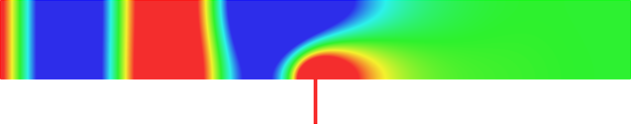
We represent the total field (acoustic pressure) in a waveguide for a wave incoming from the left.
The waveguide differs from the reference strip \(\mathbb{R}\times(0;1)\) only by the presence of a thin cavity of length \(L\).
And we vary \(L\).
In general, the propagation of the incident wave through the structure is almost not perturbed by the thin cavity: the reflection and transmission coefficients satisfy \(R\approx 0, T\approx 1\).
But we can prove that for some particular \(L=L_{\star}\), closed to a resonant length of the thin cavity, energy is completely backscattered (\(|R|=1, T=0\)).
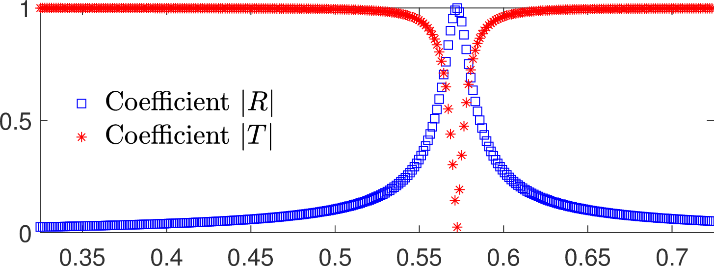
This is observed on the curves below which represent the modulus of \(R\) and \(T\) with respect to \(L\).
On the last picture, we display the total field for some \(L=L_{\star}\) such that \(|R|= 1, T= 0\). We indeed observe that the transmitted field is evanescent.
In this geometry, everything happens as if the waveguide were obstructed though there is nothing inside!

Above, we represent the total field (acoustic pressure) in a waveguide with an obstacle for a wave incoming from the left. It is a movie with respect to the time (time harmonic regime). Due to the presence of the big obstacle, there is a large reflection and the transmission is relatively weak. Now below we add a thin cavity of length \(L\) to this geometry. We can prove that there is \(L=L_{\star}\), closed to a resonant length of the thin cavity, such that the reflection and transmission coefficients satisfy \(R=0\) and \(|T|=1\). In this case, the backscattered field is evanescent. In other words, the thin cavity anihilates the reflection due to the big obstacle. Symmetry of the geometry with respect to the vertical axis is essential in this result. The last movie represents the incident wave in the reference strip \(\mathbb{R}\times(0;1)\) without obstacle.


A thin cavity can also anihilate the reflection due to a big obstacle
Above, we represent the total field (acoustic pressure) in a waveguide with an obstacle for a wave incoming from the left. It is a movie with respect to the time (time harmonic regime). Due to the presence of the big obstacle, there is a large reflection and the transmission is relatively weak. Now below we add a thin cavity of length \(L\) to this geometry. We can prove that there is \(L=L_{\star}\), closed to a resonant length of the thin cavity, such that the reflection and transmission coefficients satisfy \(R=0\) and \(|T|=1\). In this case, the backscattered field is evanescent. In other words, the thin cavity anihilates the reflection due to the big obstacle. Symmetry of the geometry with respect to the vertical axis is essential in this result. The last movie represents the incident wave in the reference strip \(\mathbb{R}\times(0;1)\) without obstacle.
Propagation through a thin slit
We represent the total field (acoustic pressure) in a waveguide which is the union of two unbounded half strips connected by a thin slit.
We send a plane from the left and we vary the frequency \(\omega\).
In general, almost no information passes through the thin slit and the energy is almost completely backscattered: the reflection and transmission coefficients are such that
\(|R|\approx 1, T\approx 0\).
But we can prove that for one particular \(\omega=\omega_{\star}\), closed to a resonant frequency of the thin slit, energy is almost completely transmitted (\(R=0, |T|=1\)).
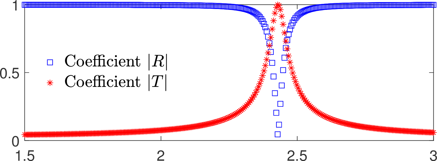
This is observed on the curves below which represent the modulus of \(R\) and \(T\) with respect to \(\omega\).
On the last picture, we display the scattered field for the particular frequency \(\omega=\omega_{\star}\) such that \(R=0, |T|=1\).
We indeed observe that the backscattered field is evanescent.

The obstacle is centered in the vertical direction. Figures left represent the \(k\) spectrum in the complex plane of the Laplace operator with Neumann boundary conditions obtained using Perfectly Matched Layers (PMLs). Bottom left is a zoom on top left. Trapped modes appear at the eigenfrequency \(k_0\) in red. On the other hand, we solve the scattering problem \(\Delta u+k^2u=0\) + Neumann B.C. for an incident plane wave at the frequency in green. The real part of the field is displayed above. We observe that nothing particular happens for \(k\) in a neighbourhood of \(k_0\). The blue dots correspond to the discretization of the continuous spectrum and to complex resonances. PMLs explain why the continuous spectrum is rotated.


The obstacle is slightly shifted in the vertical direction (5%). The eigenfrequency \(k_0\) which was embedded in the continuous spectrum becomes a complex resonance (in magenta) which is unveiled by the PMLs. We observe a rapid variation of the solution to the scattering problem for \(k\) in a neighbourhood of \(k_0\). This variation gets even faster as the imaginary part of the complex resonance is small. More details in [PDF] [PDF] .
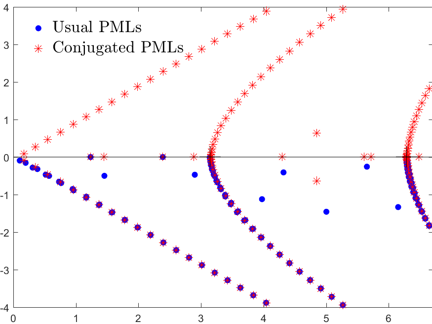
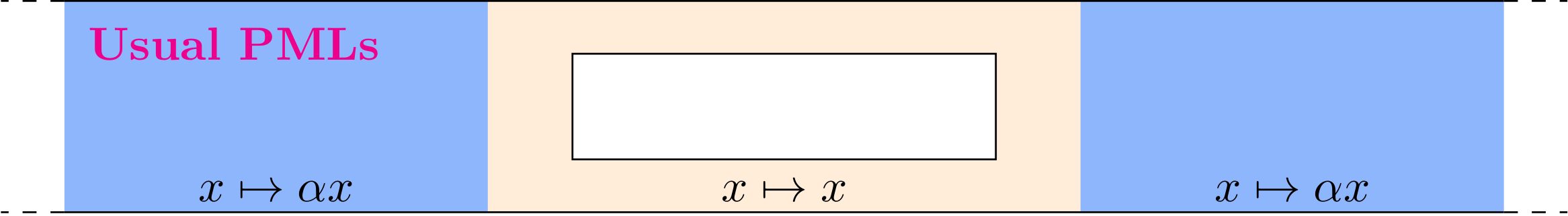
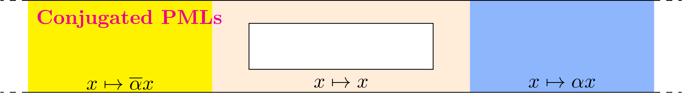
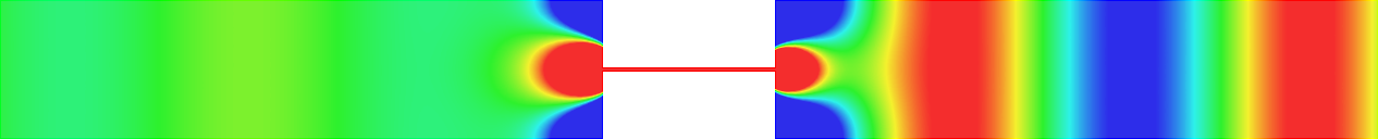
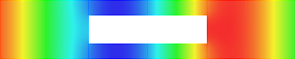
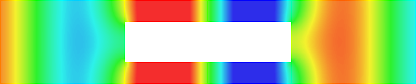
Figures left represent the \(k\) spectrum in the complex plane of the Neumann Laplacian with two kinds of Perfectly Matched Layers (PMLs). The blue spectrum has been obtained using classical PMLs to select fields which are outgoing at infinity. The red spectrum has been obtained using conjugated PMLs to select fields which are ingoing in the left lead and outgoing in the right lead. Real eigenvalues which belong to both spectra correspond to trapped modes (eigenfunctions 1 and 3 below). Real eigenvalues which are in the spectrum with conjugated PMLs but not in the spectrum with usual PMLs correspond to reflectionless modes (eigenfunctions 2 and 4 below). For the latter eigenfrequencies, there is an incident field ingoing in the left lead whose energy is completely transmitted through the structure. More details in [PDF].


 \(k=1.24\)
\(k=1.45\)
\(k=2.39\)
\(k=2.89\)
\(k=1.24\)
\(k=1.45\)
\(k=2.39\)
\(k=2.89\)
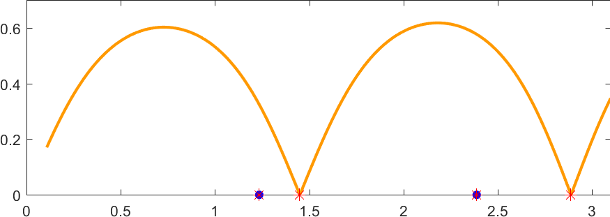 To check the results, we computed the reflection coefficient of the solution to the scattering problem \(\Delta u+k^2u=0\) + Neumann B.C. for an incident plane wave at the frequency \(k\in(0;\pi)\) (monomode regime).
The curve \(k\mapsto |R(k)|\) is displayed in orange.
We observe that \(R\) vanishes for two frequencies corresponding to the ones (\(k=1.45\) and \(k=2.89\)) which have been obtained solving the eigenvalue problem with conjugated PMLs.
To check the results, we computed the reflection coefficient of the solution to the scattering problem \(\Delta u+k^2u=0\) + Neumann B.C. for an incident plane wave at the frequency \(k\in(0;\pi)\) (monomode regime).
The curve \(k\mapsto |R(k)|\) is displayed in orange.
We observe that \(R\) vanishes for two frequencies corresponding to the ones (\(k=1.45\) and \(k=2.89\)) which have been obtained solving the eigenvalue problem with conjugated PMLs.
Below we superimpose the two spectra with usual PMLs and with conjugated PMLs for a range of \(L\), \(L\) being the width of the brick in the waveguide.
Below we show examples of reflectionless modes in two different geometries. Reflectionless modes are particular combinations of incident propagating waves for which all the energy passes through the structure without reflection. They have been computed using the method above with conjugated PMLs. For each case, we display the mode in the geometry of interest and in the reference strip.


Another geometry where \(R=0\) and \(T=1\). More details in [PDF].

In the example below, we played with the height of the thin chimneys. More details in [PDF].

Fano resonance in waveguides
The obstacle is centered in the vertical direction. Figures left represent the \(k\) spectrum in the complex plane of the Laplace operator with Neumann boundary conditions obtained using Perfectly Matched Layers (PMLs). Bottom left is a zoom on top left. Trapped modes appear at the eigenfrequency \(k_0\) in red. On the other hand, we solve the scattering problem \(\Delta u+k^2u=0\) + Neumann B.C. for an incident plane wave at the frequency in green. The real part of the field is displayed above. We observe that nothing particular happens for \(k\) in a neighbourhood of \(k_0\). The blue dots correspond to the discretization of the continuous spectrum and to complex resonances. PMLs explain why the continuous spectrum is rotated.
The obstacle is slightly shifted in the vertical direction (5%). The eigenfrequency \(k_0\) which was embedded in the continuous spectrum becomes a complex resonance (in magenta) which is unveiled by the PMLs. We observe a rapid variation of the solution to the scattering problem for \(k\) in a neighbourhood of \(k_0\). This variation gets even faster as the imaginary part of the complex resonance is small. More details in [PDF] [PDF] .
Conjugated PMLs in waveguides
Figures left represent the \(k\) spectrum in the complex plane of the Neumann Laplacian with two kinds of Perfectly Matched Layers (PMLs). The blue spectrum has been obtained using classical PMLs to select fields which are outgoing at infinity. The red spectrum has been obtained using conjugated PMLs to select fields which are ingoing in the left lead and outgoing in the right lead. Real eigenvalues which belong to both spectra correspond to trapped modes (eigenfunctions 1 and 3 below). Real eigenvalues which are in the spectrum with conjugated PMLs but not in the spectrum with usual PMLs correspond to reflectionless modes (eigenfunctions 2 and 4 below). For the latter eigenfrequencies, there is an incident field ingoing in the left lead whose energy is completely transmitted through the structure. More details in [PDF].
\(k=1.24\)
\(k=1.45\)
\(k=2.39\)
\(k=2.89\)
To check the results, we computed the reflection coefficient of the solution to the scattering problem \(\Delta u+k^2u=0\) + Neumann B.C. for an incident plane wave at the frequency \(k\in(0;\pi)\) (monomode regime).
The curve \(k\mapsto |R(k)|\) is displayed in orange.
We observe that \(R\) vanishes for two frequencies corresponding to the ones (\(k=1.45\) and \(k=2.89\)) which have been obtained solving the eigenvalue problem with conjugated PMLs.
Below we superimpose the two spectra with usual PMLs and with conjugated PMLs for a range of \(L\), \(L\) being the width of the brick in the waveguide.
Below we show examples of reflectionless modes in two different geometries. Reflectionless modes are particular combinations of incident propagating waves for which all the energy passes through the structure without reflection. They have been computed using the method above with conjugated PMLs. For each case, we display the mode in the geometry of interest and in the reference strip.
Invisibility in waveguides
- Perfect invisibility. We represent the total field (acoustic pressure) in the reference geometry (bottom) and in the pertubed waveguide (top). At \(x=\pm\infty\) in the perturbed waveguide, the field is the same as in the reference geometry. The reflection coefficient \(R\) and the transmission coefficient \(T\) satisfy \(R=0\), \(T=1\). More details in [PDF].
Another geometry where \(R=0\) and \(T=1\). More details in [PDF].
In the example below, we played with the height of the thin chimneys. More details in [PDF].
- Complete reflectivity. We represent the total field (acoustic pressure). The goemetries have been designed so that \(T=0\). All the energy is backscattered. More details in [PDF].
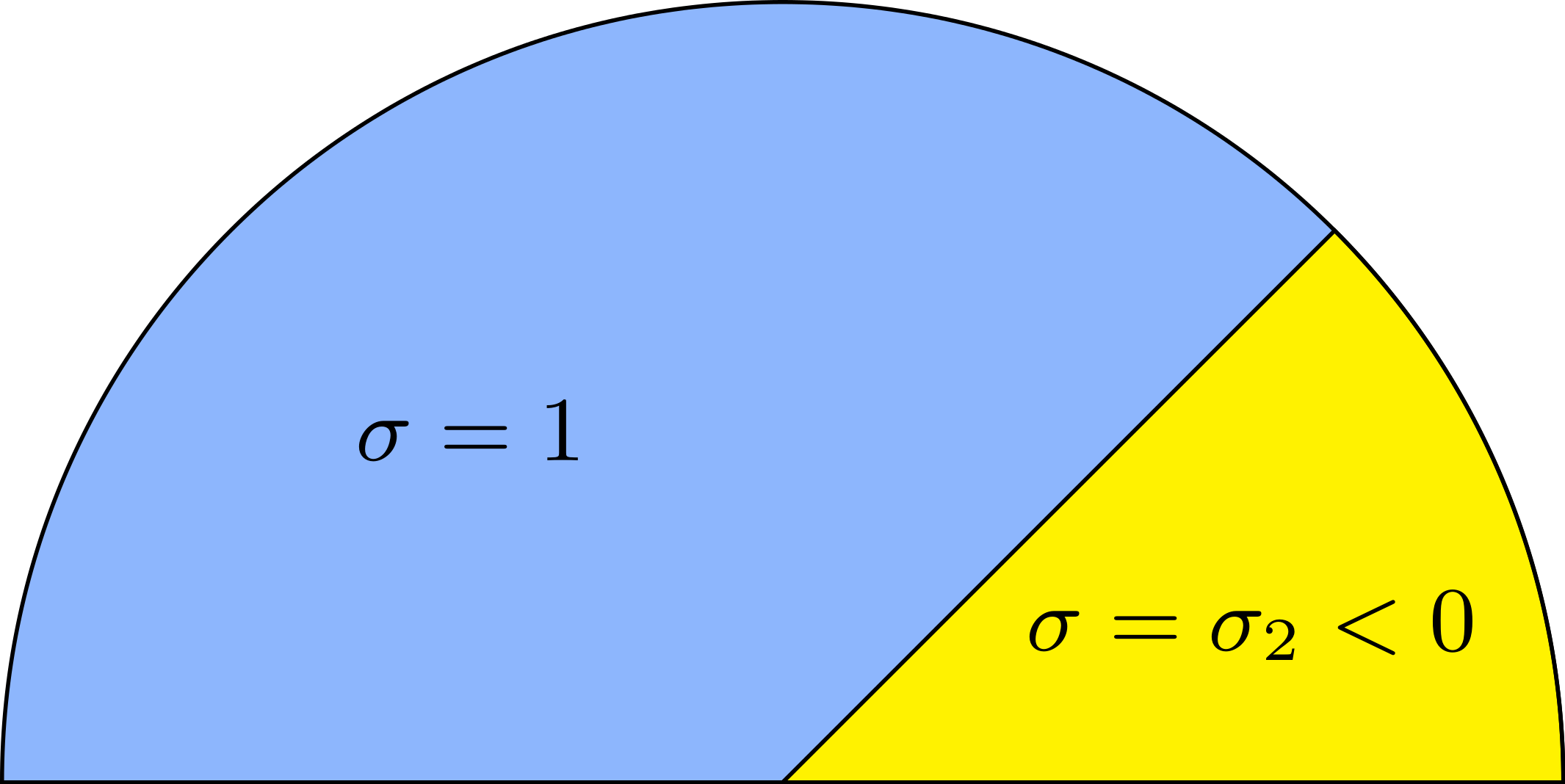
Plasmonic and metamaterials
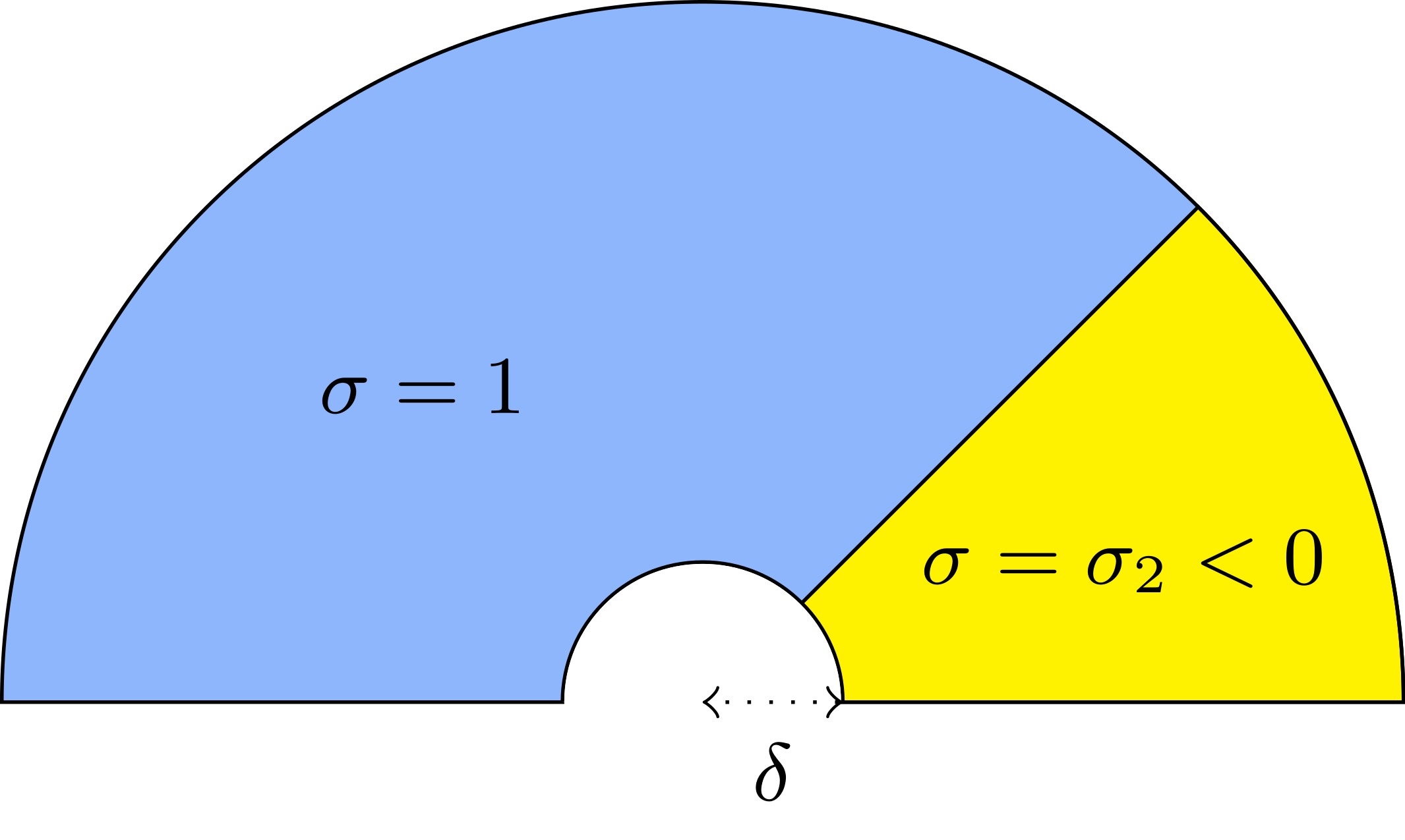
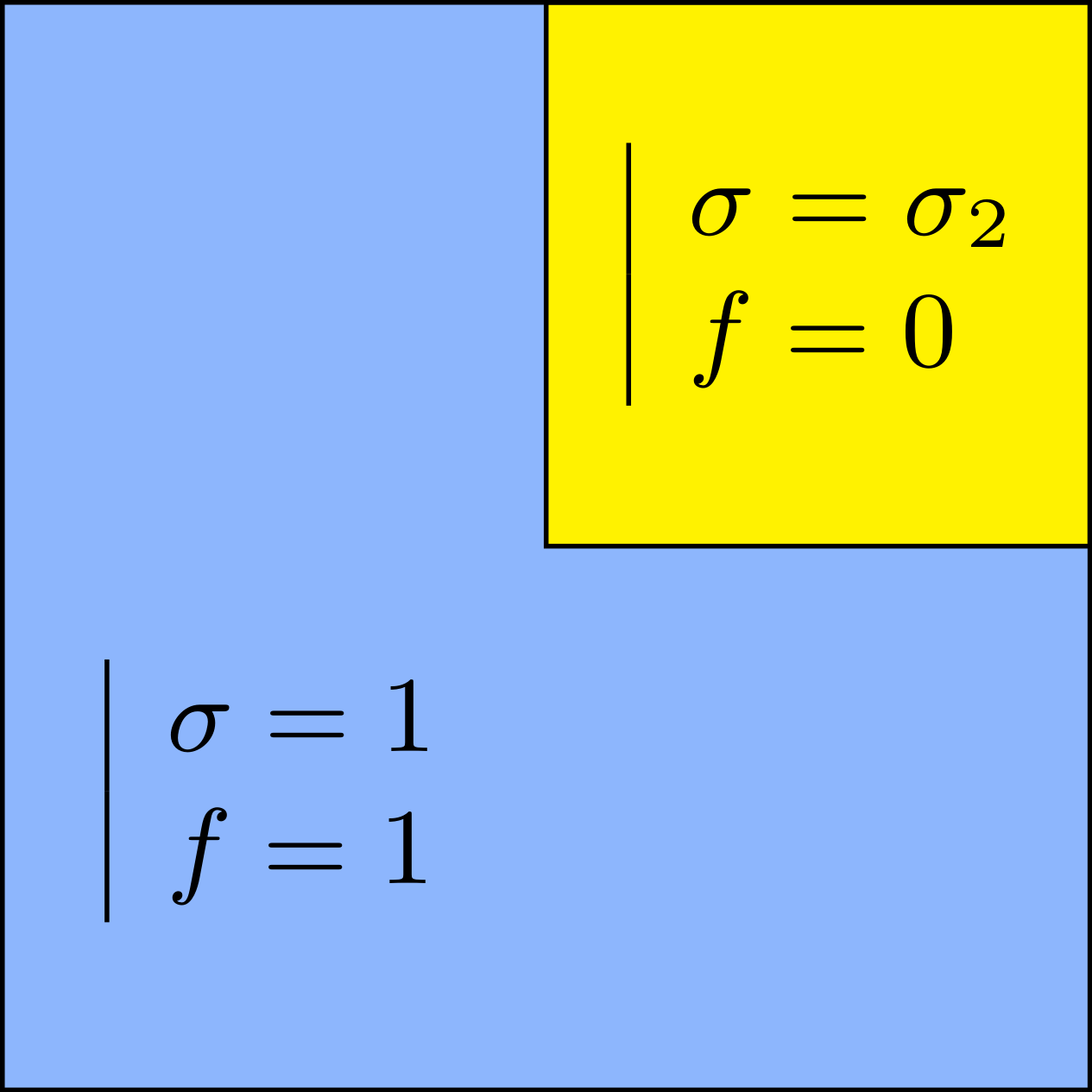
We consider the problem\begin{array}{|rl} -\mbox{div}(\sigma\nabla u)=f &\mbox{ in }\Omega\\ u=0&\mbox{ on }\partial\Omega \end{array}
with a sign changing \(\sigma\).- Singular behaviour. For certain values of \(\sigma\), very singular behaviours can appear which are not met with positive materials. Here we represent \(t\mapsto \Re e\,(u(x,y)e^{-i\omega t})\) for a given \(\omega>0\). Everything happens like if a wave was absorbed by the corner. The wave propagates to the corner but never reaches it. We talk about "black-hole phenomenon". More details in [PDF], [PDF].
- Rounded corner. The solution can be very sensitive to the geometry. Here we represent \(\delta\mapsto u^{\delta}\) as \(\delta\to0\), where \(\delta\) is the radius of the inner circle. More details in [PDF], [PDF].
- Mesh refinement. We solve numerically the above problem with a usual P1 finite element method for different meshes (we refine the mesh).
For \(\sigma_2/\sigma_1\in[-3;-1/3]\), in general the solution does not converge (below left \(\sigma_2=-1.0001\)).
For \(\sigma_2/\sigma_1\in(-\infty;0)\setminus[-3;-1/3]\), the solution does converge (below right \(\sigma_2=-3.001\)). More details in [PDF].
![[CSS valide]](http://jigsaw.w3.org/css-validator/images/vcss)